Tentative laboratory
topics
Aug. 22: Pendulum measurement of "g"
Week 1 homework
Aug. 29: Gravity - a function of elevation (Field).
Download gravity data here
No lecture or lab on Labor Day. There might be room for volunteers to
assist with a field project.
Sept. 12: Field gravity measurements (Field).
Gravity data: locations, elevations and dial
readings. Do not use GPS elevations, use values next to dial readings.
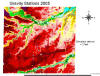 Image (click to enlarge): New gravity stations (yellow triangles) on LIDAR
data, color classified at 2-foot intervals. Blue is low, dark brown is
high, with green and yellow intermediate. Can you pick out any geographic
features?
Image (click to enlarge): New gravity stations (yellow triangles) on LIDAR
data, color classified at 2-foot intervals. Blue is low, dark brown is
high, with green and yellow intermediate. Can you pick out any geographic
features?
You have everything you need to calculate the simple Bouguer gravity
values for the 4 new stations, please use the 1930 IGF and 2,670 kg/cubic meter
for your reductions.
Previously collected gravity data and other useful stuff
2-D Talwani spreadsheet
Sept. 19: Gravity data reductions and interpretation (computer lab).
Sept. 26: Field magnetometer survey.
Oct. 3: Magnetic data processing (computer lab)
Magmodel - a
spreadsheet that calculates the total field anomaly due to a buried dipole.
DATA - downloaded last
Wednesday. "Save as" to your storage media and make a series of Surfer
maps as per instructions. Remember, make one contour map using all data of
each kind (top sensor, bottom sensor, gradient - 3 contour maps in all) and a
second contour map of each type after you have removed high-amplitude spikes
(positive and/or negative) from the data (not just from the grid).
Note: a spike on the lower sensor does not necessarily mean a spike on the top
sensor (although the gradient will spike - after all, gradient is simply top
minus bottom divided by distance between them - or is it bottom minus top?
Another issue: Top sensor data should be a lot smoother than bottom sensor
data. Is it possible that the top/bottom are reversed? The last
profile may have lots of noise on the bottom sensor if the metal decorations on
the operator's belt were magnetic.
See this page
for an example of a magnetometer report. Links on the page direct you to
figures.
Oct. 10: Ground-penetrating radar (Field)
Oct. 17: Autumn Break – no lecture or 4610 lab, probably will have field
research expedition (willing workers welcome!).
October 24: Synthetic seismograms.
Spreadsheet that does convolution.
Note that one sheet generates a wavelet - you can change the frequency, then
copy and 'paste as' values into column A on the Series
page. Please allow the macros to be activated, else the program
will not run. Put your reflection coefficient time series in Column B,
then hit the Run button for the convolution, which should appear in
Column C. Set up to graph C(t) as a function of T (this may take some
copying/past or generating cell addresses on the third page - insert additional
pages for the graph if necessary). My guide has not been updated to
reflect improvements in the spreadsheet so, where conflicts exist, use the
wavelet from the spreadsheet rather than the wavelet from the handout.
Also, compare and contrast synthetic seismograms using low-frequency and
high-frequency wavelets, once reflections from the base of the thin bed begin to
seriously degrade the reflection from the top of the page. Do not use
frequencies greater than 100 hz or less than 10 hz.
Oct. 31: Reflection seismograms, interpretation.
Nov. 7: There will be no lab on the afternoon of Nov. 7 (Midterm -
take-home, open book, distributed Monday at 9 AM, due Tuesday at 10 AM).
Friday, Nov. 11 Veterans' Day - NOTE!! Seismic refraction - our
annual Veterans' Day turkey shoot - we spend all day at a remote field
research site - TBA.
Nov. 14: Seismic refraction interpretation (computer lab)
Seismic refraction
interpretation software
Nov. 21: Lecture AM, perhaps a video for lab.
Nov. 28: Earthquake seismograms I
Dec. 5: Earthquake seismograms II
FINAL EXAM (if needed): Tuesday, December 13, 10:15 – 12:15.
Formal report or short report?
ORGANIZE AND USE YOUR TIME PROPERLY. Laboratory reports take a lot of
time. You cannot hope to complete an entire report (data analysis to written
draft) overnight. I cannot do that, and I know all of the tricks
and shortcuts. Your data analysis and graphs should be completed within 48
hours of the fieldwork, and a rough draft should be completed no less than 48
hours prior to the deadline. If you seek help with data processing on a
Monday morning and the report is due that Monday afternoon, it will be clear to
me that you did not begin report preparation according to instructions.
You should put this draft aside over night, reread it carefully and
critically, and pencil in editing changes right on the hard copy. Did you really
mean what you wrote, and did you write what you need to communicate? Is each
graph necessary and does it have an informative caption? Is it properly
numbered? Is your abstract informative and concise? At this point, rewrite your
report and make those necessary revisions. Then FILE YOUR FIRST DRAFT (keep it
handy, do not throw it away). Logjams will occur if everyone delays report
writing until the last minute. I am often unavailable the day before a report is
due - you should come to me with questions while doing that first draft! In the
professional world, reports are needed so that decisions can be made, bids
submitted, plans finalized and budgets drafted. A late report may require a
client to proceed without benefit of what we were supposed to be able to tell
him, for which he might sue for failure to fulfill the contract. It is your
responsibility to make timely use of the resources at your disposal - including
your time.
Late reports distract you and me from concentrating on current topics. This
is not efficient.
Return to Syllabus

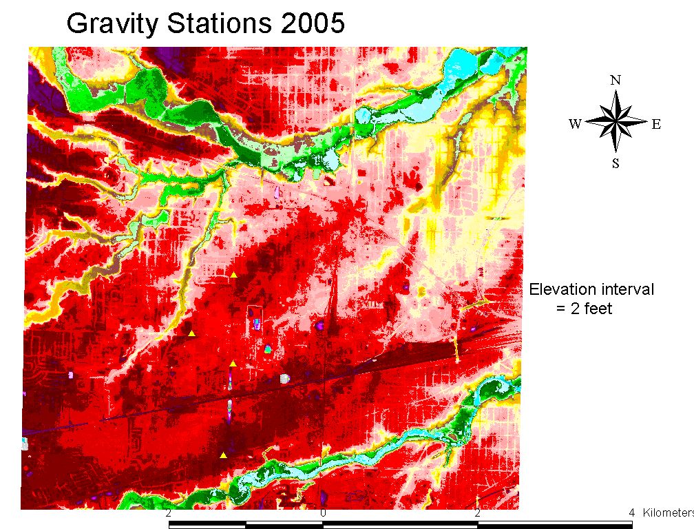 Image (click to enlarge): New gravity stations (yellow triangles) on LIDAR
data, color classified at 2-foot intervals. Blue is low, dark brown is
high, with green and yellow intermediate. Can you pick out any geographic
features?
Image (click to enlarge): New gravity stations (yellow triangles) on LIDAR
data, color classified at 2-foot intervals. Blue is low, dark brown is
high, with green and yellow intermediate. Can you pick out any geographic
features?