A
SMALL DOSE OF STATISTICS
Dr.
“A man with one watch knows what time it
is. A man with two watches is never
quite certain.”
We
have a similar problem with geographical coordinates supplied by a GPS
receiver. As you stood in one location,
latitude, longitude and elevation kept changing. No, plate tectonics was not responsible for
this apparent motion. One problem
associated with measurements is uncertainty,
or error. By “error” I do not mean mistakes or
incorrectness. “Error” in this context
refers to the degree of uncertainty.
For
example, a friend with a simple GPS receiver informs you where her seat in the
Glass Bowl is located in terms of latitude and longitude. If you set your GPS unit to navigate to that
location, how close will you get? Inside the stadium? In the correct section?
Within ten seats or rows? Within two seats or rows? Can you identify her seat by means of
latitude and longitude alone, or does GPS technology lack that degree of
accuracy? The difference between the
true location and your GPS location is the error.
During
a field GPS lab, students used Trimble GeoExplorer II
GPS receivers to collect location information.
These locations were stored in GEII memory, downloaded to computers, and
differential corrections calculated.[1] You have lists, provided by the teaching
assistant, of corrected and uncorrected locations. Instead of latitude and longitude, these
locations are listed in terms of “military grid”, or UTM (Universal Transverse
Mercator), a Cartesian (X and Y axes at right angles to one another) system
many find more convenient for local maps than latitude and longitude. What is the best value you can write for each location where GPS
readings were collected?
Errors
can be either systematic or random.
A systematic error involves a bias of some kind. For example, a medical scale improperly set
such that an empty platform weights 1.1 kg will yield measurements that are
consistently 1.1 kg more than the true weights of individuals who use that
scale. Measuring devices used in commerce
(for example: supermarket scales use to weight meat and produce and gasoline
pumps) are checked and certified accurate by local government officials to
protect consumers. A gasoline pump that
delivers 5% less gas than indicated cheats the customer out of one gallon for
every twenty one gallons purchased.
Random
errors involve scatter. A baker
producing bread listed as twenty ounces per loaf has difficulty making each
loaf such that it weights precisely twenty ounces. Some loaves are a little bit heavier, some might be a little bit lighter. If loaves sold customers average twenty
ounces in weight, on a given day one family might get less bread for their
money than another family. However, if
the variations in weight are truly random and there is no effort made to select
heavy loaves, customers are not at a disadvantage because loaves that are too
light are balanced out by loaves that are too heavy. However, systematic error might also occur at
the bakery. A baker setting out to cheat
customers might modify his recipie such that only the
heaviest loaves weight twenty ounces, while a baker concerned with legal or
public relations consequences of selling underweight bread might see to it that
all loaves weigh over twenty ounces.
Before
discussing statistical methods for dealing with measurements, it is useful to
discuss the concept of probability. If there are several equally likely, mutually
exclusive, and collectively exhaustive outcomes of an experiment, the
probability p of an event E is

For example, when flipping a coin, there are two
mutually exclusive, collectively exhaustive outcomes possible: heads and
tails. The outcome will be either heads
or tails (mutually exclusive) and there is no possible outcome other than heads
or tails (collectively exhaustive).[2] If a coin and coin flipper are unbiased,
there is an equal probability of either outcome. How can we determine the probability of a
more complex outcome - for example, the probability of obtaining 3 straight “heads”?
On
the first flip, heads (H) and tails (T) are equally probable. There is one possible favorable outcome (H)
out of two possible outcomes total. Each
flip has either (H) or (T) as a possibility.
What combinations are possible in 3 flips of the coin? HHH, HHT, HTH, HTT, TTT, TTH, THT, THH are
the only possible outcomes of 3 flips of the coin. 1 favorable outcome out of 8 possible
outcomes: p = 1/8; 0.125 or 12.5%.
What
is the probability of 2 consecutive heads in 3 flips? p = 3/8;
0.375 or
37.5%.
Now
let’s play cards. We’ll use a standard
deck of 52 cards (no jokers). The
probability of drawing a specific card (ace of diamonds) is 1 in 52. The probability of drawing any ace is 4 in
52. What is the probability of drawing
two aces from the deck in the first two consecutive draws?
The
probability of drawing the first ace is 4 in 52. The probability that the second card drawn
from the deck is an ace is 3 in 51 if the first card drawn was an ace. If the first card drawn was not an ace, the
probability of drawing an ace in the second draw is improved to X in 51, but
chances for a favorable outcome (pair of aces) has already vanished. We obtain the probability of a compound event
(A and B) by multiplying the
probabilities of each event:

What
are the odds of 3 straight wins in roulette?
The wheel has 37 slots, with each outcome equally probable (we assume an
honest game).

Casinos
are profitable for the operators because probability in on the side of The
House for all casino games, even when played honestly.[3] The only casino game where players can win in
the long run is Black Jack, and then only if a player can keep track of cards
played from the shoe. By counting how
many of certain cards have been dealt, card counters can improve their take by
betting heavily when the deck is rich in cards unfavorable to the house. Of course, casinos prohibit card counting and
eject players who appear to be card counting (in other words, regular winners
at the black jack table).
Exercises:
1. Calculate the probability of winning the Ohio
Lottery. You must select the 6 numbers
drawn from a set of 47.
2. Calculate the probability that none of the 6 numbers you select are
among the 6 selected as the winning set.
How many students in the class arrive at the same probability?
---------------------------------------------
It
is not our objective to become experts in probability theory. There are probably courses offered by the
Mathematics Department that focus on probability and statistics. We need to develop some knowledge of
statistical jargon (specialized terms) and a bit about their meanings.
The
average value, or mean, is equal to
 (1)
(1)
where
v are values and n equals the number of values (the ∑ symbol means
"sum"). The median is the value in the center, half
of the values are higher, and half are lower.
It is often better to specify the arithmetic
mean rather than say average - average
is less rigorously defined.
Example:
the average of the series S = {5, 7,
8, 4, 7, 6, 10, 7, 4} is 58/9 = 6.44.
The
median value is the middle
value. Half of the values are higher,
and half are lower. The median of series
S is 7 (4, 4, 5, 6 are lower than,
and 7, 7, 8, and 10 are equal to or higher than, 7).
The
mode is the most frequent
value. The mode of series S is 7.
The
range of a set of values is the
difference between extreme values (highest and lowest) plus 1. The range of series S = (10 - 4 + 1) = 7.
Variance is a measure of the dispersion
a set of values. The variance of a population (σ2) is
defined as
 (2)
(2)
where
N
is the number of members of the population, μ is the mean value, and Xi is the value of the ith member. The variance
of a sample (s2)
is defined as
 (3)
(3)
where  is the mean of the
sample, and n is
the number of values in the sample.
It
is my understanding that a "population" involves all (for example,
all residents of
Random
errors scattered about a mean frequently exhibit a normal distribution. There
are more values close to the mean than far from the median. A normal distribution describes data or
measurements that are consistent with the equation
 (4)
(4)
where
u is the value of the function, μ
is the mean (equation 1), and σ is the standard deviation (equation 5 or equation 6).
 (5)
(5)
 (6)
(6)
Of course, s replaces σ when characterizing a sample rather than
a population.
 Equation 4 describes the bell curve, the graph consistent with
a normal distribution.
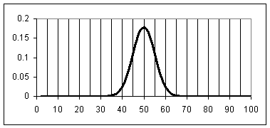
Figure 1: bell curve for mean = 50 and standard
deviation = 5.0.
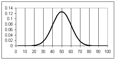
Figure 1 is an example of a bell curve. Compare Figure 1 with Figure 2, a distribution
with the same mean but a larger standard deviation.
 Figure
2:
The area
under a segment the bell curve represents the percentage of a population or
sample that falls within the range of that segment. The area between the mean and one standard
deviation above or below the mean equals 34.13% of the total area. The area between the mean and two standard
deviations equals 47.72%, and the area between the mean and three standard
deviations equals 49.87%.
Given a set of
measurements subject to random error, the standard deviation provides a measure
of the confidence we might have that the "true" value lies within a
certain range. Confidence is 68% that
the true value lies within 1 standard deviation of the
mean (in Figure 2, between the values 40 and 60). Confidence is 95% that the true value lies within 2 standard deviations (between 30 and 70 in
Figure 2) and 99% that it lies within 3 standard deviations (between 20 and
80).
Most "scientific"
calculators have built-in statistical functions. You will probably have to locate the manual
and look up the procedure for entering data and accessing the results (mean,
standard deviation).