Resistivity is measured by planting 2 sets of electrodes into the earth. Via one set, a measured electrical current is transmitted into the ground. A second set is used to monitor changes in the potential induced by this current. The general form of equations relating resistivity to current and induced voltage is

(2-1)   

where "G" is determined by the geometry of the array (array: spatial deployment of electrodes). V and I are measured using a voltmeter (or potentiometer) and ammeter respectively. The arrays we most frequently use are collinear - that is, the 4 electrodes lie in a straight line. There are configurations that are not collinear but I use those only when the situation so demands.

Wenner array: the Wenner array geometry is depicted in Figure 1. Throughout this discussion, electrodes A and B refer to current electrodes (usually metal stakes) and electrodes M and N refer to potential electrodes (usually porous pots).

Figure 1: Wenner array.

In the Wenner array, distances AM = MN = NB = "a-spacing".

Suppose the earth were a uniform, homogeneous, isotropic half-space (from this point, all "uniform" structures are homogeneous and isotropic). It is not difficult to compute the potential field set up by this array relating the resistivity of the earth to the array geometry

(2-2)   

Consider next an earth that is not uniform, but is instead composed of a single uniform layer over a uniform half-space. If the aperture (electrode spacing) if the array is small compared to the thickness of the layer, the array does not "see" the underlying half-space and measured the true resistivity of the layer. If, on the other hand, the array is very large with respect to the thickness of the surficial layer, the array samples the half-space rather than the layer and measures the true resistivity of the half-space. If the array dimension is about the same as the layer thickness, an intermediate value is measured. Equation 2-2, however, is calculated based on the response of a uniform earth. Hence, we do not call this value the resistivity of the earth but, rather, the APPARENT RESISTIVITY (ρ_a). Resistivity is calculated as if the earth were a homogeneous, isotropic half-space, using Equation 2-2.

We interrogate the earth by increasing the a-spacing and measuring apparent resistivity at various spacings. Data are plotted on LOG-LOG graph paper, apparent resistivity on the vertical axis as a function of electrode spacing. For the Wenner array, electrode a-spacing is usually used as the independent (horizontal, or X-axis) variable. These data define a SOUNDING CURVE (Figure 2). An electrical sounding is a survey in which we interrogate more and more deeply by measuring apparent resistivity ρ_a as a function of electrode spacing AB/2 or "a".

Figure 2: Sounding curves for Wenner and Schlumberger arrays.  Note use of log-log graph paper.

Interpretation will be discussed shortly. Edwards (1977) developed the concept of EFFECTIVE DEPTH, Z_E, the interval within the subsurface of a homogeneous earth that contributes 50% of the signal. For the Wenner array, the center of this effective depth is given by

(2-3)   

(Edwards, 1977) where "a" is the "a-spacing" of the electrodes. In other words, if the a-spacing for a given measurement is 10. meters, 50% of the signal is controlled by a zone centered about 5.2 m below the surface, and the effective depth zone extends from 0.5 Z_E to 1.6 Z_E (from about 2.6 m to about 8.3 m). In order to probe the earth, we begin with short a-spacings, make the measurements of I and V, and expand the array by increasing "a" in a systematic manner. Data are plotted on the log-log graph (ρ_a as a function of "a") generating the sounding curve.

In the field, a typical a-spacing for the first measurement is 2.0 meters. This means each potential electrode is place 1.0 m from the sounding point and each current electrode is placed 3.0 m from the sounding point. It is generally a good idea to obtain 5 evenly spaced data points per log cycle. This means a = 2.0, 3.2, 5.0, 7.9, 13, 20, 32, 50, 79, 130, and so on until sufficient sampling depth has been achieved (or until you run out of wire). Note that these values represent 10^0.7, 10^0.9, 10^1.1, 10^1.3 and so on. For the Wenner array, the distance from the sounding point to each potential electrode is a/2 and the distance to each current electrode is 1.5*a. The decision as to "How large an 'a' is enough?" (how far should we go?) depends on the specific geologic problem. This will be discussed below.

The Schlumberger array (Figure 3) resembles the Wenner array. The main difference in terms of deployment geometry is the distance between potential electrodes (MN) is not held to half the distance between the current electrodes (AB) as in the case of the Wenner array. Apparent resistivity calculations are slightly more complex:

(2-4)  

and the data plotted are apparent resistivity as a function of AB/2. We are using a symmetric Schlumberger array, one in which electrodes are symmetrical about the sounding point. There are variations (see Parasnis, pp. 189-190 for an example) on the Schlumberger array that can be used for PROFILING (seeking lateral rather than vertical variations in electrical properties). 

Figure 3: Schlumberger array with current electrodes A and B, and, potential electrodes M and N.

One restriction on use of the Schlumberger array: electrode separation AB must be at least 5 times separation MN;

(2-5) AB > 5 * MN

for Equation 2-5 to be valid (again, from potential field theory "It can be shown that - - " but you will have to accept this ex cathedra rather than have me go through the mathematical proof). Effective depth midrange Z_E is about

(2-6) Z_E/L = 0.190

(Edwards, 1977) where "L" is distance AB, and the 50% sample zone extends from 0.5 to 1.6 Z_E. Note that with the Wenner array I defined Z_E in terms of dimension "a", which is 0.66 * AB/2, or one-third of AB (AB = L). Thus, effective depth for a given AB in the Wenner case is 0.519/3, or 0.173*L. The Schlumberger provides, for a given spacing of current electrodes, about 10% greater interrogation depth than that provided by the Wenner array.

As with the Wenner array, we begin a sounding with a short AB/2 and expand in "log" steps. I begin with AB/2 = 2.5 m and MN/2 = 0.5 m (remember Equation 2-6). At 5 data points per log cycle, the array expands as follows: 2.5, 4.0, 6.3, 10, 16, 25, 40, etc. (note that these are 10^0.4, 10^0.6, 10^0.8, 10¹, 10^1.2 and so on). Potential electrodes MN are moved only when potential drops become too small to measure with sufficient precision. In a typical survey, it may not be necessary to increase the MN/2 distance until AB/2 is 10. meters. At this point, we measure (V/I) for both the old MN/2 value (0.5 m) and for the new MN/2 (10/5, or 2 m). This procedure permits us to detect near-surface heterogeneities, something not available to us with the Wenner array.

There are three significant advantages for using the Schlumberger rather than the Wenner array. First, the Schlumberger array has a slightly greater interrogation depth. Second, because the resistivity is being sampled between points MN, the lateral resolution is better for the Schlumberger array. (IMPORTANT: I have encountered engineers who think the AB distance determines lateral resolution; they are wrong. I have not found the source of this widespread error but would appreciate your informing me if you find this in print somewhere. A bit of analysis along the line of "voltage drops across resistors in series" should allow you to understand why my statement regarding MN is true.) Third, because MN and AB can be changed independently, lateral variations between the MN electrodes are detected when the Schlumberger array is used. Because both AB and MN must be moved simultaneously in making a Wenner sounding, a Wenner user can not determine if details of a curve are controlled by variations as a function of depth or by lateral variations in electrical properties.

Some investigators like to do "profiling" - that is, selecting a specific array spread (AB, MN are constant) and moving the array from point to point. This method is dangerous and is one reason (I think) the USEPA does not like electrical resistivity as much as electromagnetic (EM) when prospecting for contaminated ground water. Shallow resistivity variations not linked with conditions at depths of interest can obscure signals sought. Investigators who profile without due respect for shallow resistivity variations are likely to fail. Lateral variations in resistivity are best detected by performing soundings along a profile.

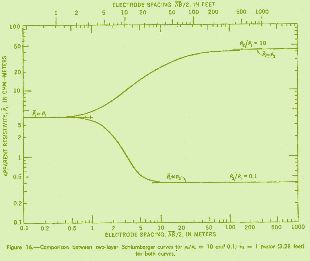
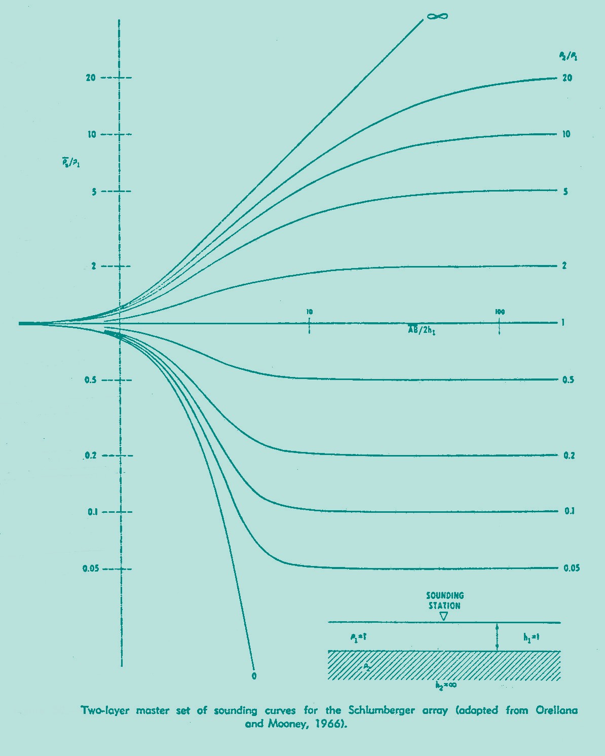
Figure 4 shows Schlumberger sounding curves for a single layer over a half-space, one curve for the layer 10 times more resistant than the half-space, the other for the layer 10 times less resistant than the half-space. Note that the layer thickness is 1 m for both cases. These curves begin to depart from the horizontal "homogeneous" line just a bit to the left of AB/2 = 1.0 m. Note that these curves do not "level out" until AB/2 is 10 to 100 times the layer thickness for this resistivity contrast (note comments on profiling, previous page). Often we can not extend a line far enough for the curve to level off; however, we can still determine the resistivity contrast (provided it is not extreme) by noting the slope of the curve. Figure 5 shows a set of "2-layer" (actually, layer over half-space) MASTER CURVES. By comparing these curves with a set of field data, we can determine the resistivity of the layer (it is equal to the horizontal line value prior to the point where the curve turns up or down) and the contrast between that layer and the underlying material - from which we then calculate the resistivity of the half-space.

Figure 4: Sounding curves for layer of half-space.

Figure 5: Master curves for layer-over-halfspace, Schlumberger array.

Example: suppose the resistivity of the top layer is 100 ohm-meters and that we note, by comparing slopes with master curves, that the underlying material is of lower resistivity and that the slope matches the 0.2 curve. This means the ratio ρ₂/ρ₁ = 0.2, or, the underlying material has a resistivity of 20 ohm-meters.

On curve matching, the point where layer thickness h = AB/2 is called the DEPTH INDEX. I use a set of these master curves on a transparent sheet - once I find a match, I can read the thickness of the layer by noting where this (h = 1) line lies with respect to my data. This value, read from the plot of my field data, gives me the thickness of the top layer.

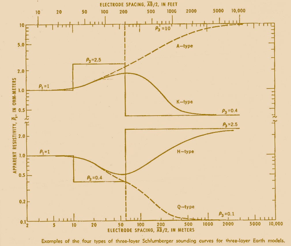
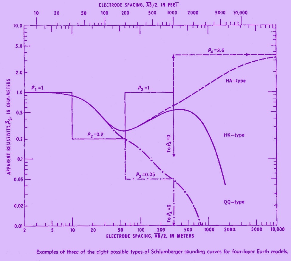
Few earth structures can be modeled as a single layer over a half- space. One more typical situation occurs when the unsaturated zone overlies a porous unconfined aquifer, which in turn overlies low- porosity bedrock. In this case, the top layer has a higher resistivity than the middle layer, which has a lower resistivity than the bedrock. Figure 6 shows the H-type curve as representing this condition. An A- type curve shows two layers over the halfspace with increasing resistivity with depth, and the K-type curve shows a high-resistivity layer between a low-resistivity layer and half-space. The Q-type curve shows two layers over a half-space with resistivity decreasing with depth. You will not be expected to recall from memory A-, H-, Q- or K- type curves. You should, however, be able to inspect a curve and draw conclusions regarding the minimum number of electrical layers and the general trend of high/low relative resistivities. Figure 7 shows further complexity: 3 layers over a half-space (4 electrical units). Later, we will use computer programs to model the electrical response of a layered earth (Program DCSCHLUM) and to interpret by inversion a Schlumberger sounding curve (Program ATO).  I have a spreadsheet that does forward models: you specify a model consisting of horizontal layers and the spreadsheet calculates the curve.  You enter the data in the appropriate cells and can see both the model curve and data on the same chart.

Figure 6: 2 layers over halfspace: 4 possible perturbations. 

Figure 7: 3 layers over halfspace, 4 of the possible 9 perturbations.

Just as the depth index offers a clue to the thickness of the top layer, inflection points offer clues to the depth to contacts between electrical units further down. For example, in Figure 2-7, note how the K- and H-type curves change slope at AB/2 distances about equal to the depth at which resistivity changes occur.

We have 1 license for a sounding inversion program titled IX1D.  The standard cost of this license is about $1000.  Running the program requires a hardware key.  Interpretations for publications (including your reports) based on resistivity soundings will utilize this resource.

Figure 8: students conducting and electrical sounding.

One final note: the slope at any point on the sound curve is a function of just two layers. You can thus evaluate your data by determining ρ₂ from the slope in the first part of the curve, then deduce ρ₃ by noting the contrast with ρ₂, and so on.

THE DIPOLE-DIPOLE ARRAY

This array is useful for mapping shallow variations both lateral and vertical simultaneously.  Select a dipole dimension ("a" - Figure 9) appropriate for the depth of interest.  According to Edwards (1977), the effective depth for the dipole-dipole array is about greater than 3a but less than 4a.  In other words, when using 10-meter dipoles, I can image the upper 12 meters or so when I make measurements between dipole separations n = 1 through n = 4.

Figure 9: Dipole-dipole array.  "n" must be an interger (1, 2, 3, etc.).

The apparent resistivity for the dipole-dipole array is

(2-7)  

and the value for each dipole-dipole combination is plotted on a pseudosection which resembles a cross section of the region under the dipole-dipole profile.  The traditional pseudosection plots apparent resistivity at the point where lines drawn downward at 45 degree angles from the center of each dipole intersect.  This traditional pseudosection exaggerates the depth of anomalous materials.  Edwards (1977) tells us how to modify the pseudosection such that it better matches true depths.  I have had good success in using coefficients Edwards (1977) published at Talgua and down-gradient from the Stringfellow site.

Disadvantages of the dipole-dipole are, first, that high electrical currents are required to interrogate deeply into the earth and, second, that true rock resistivities are not easily calculated.  Software to invert dipole-dipole resistivity profile data into a "true" cross-section showing rock resistivities (rather than apparent resistivities) is expensive.  We have one license, which cost more than the IX1D inversion program.

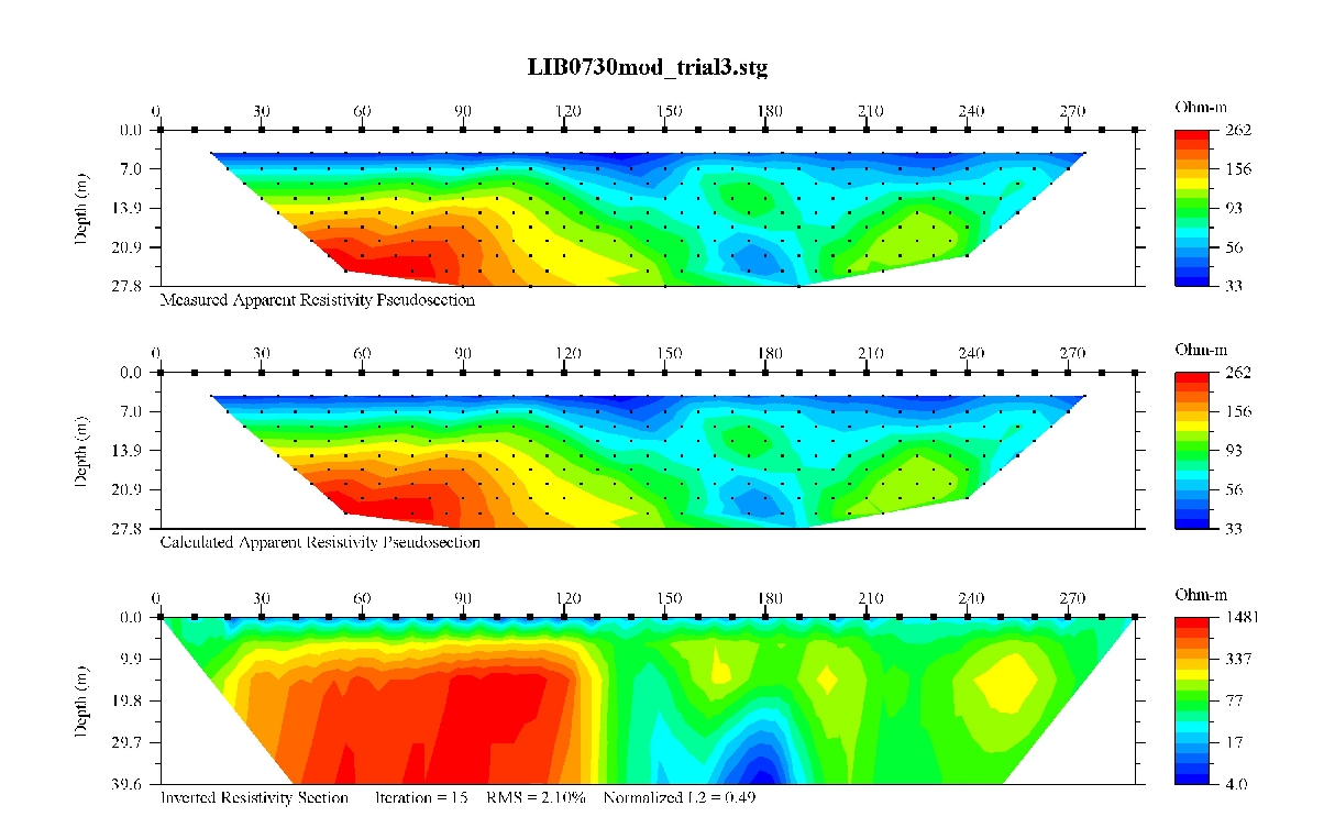Figure 10:  results of a dipole-dipole profile run in search of the edge of carbonate bedrock (high resistivity - red) at Liberty Crater.  The top pseudosection is the observed, the bottom the geological model, and the center is the pseudosection calculated for the geological model. 

ONE FINAL WARNING: potential fields are not unique. That is, there are numerous electrical resistivity structures that could yield any specific sounding curve (IX1D performs an 'equivalence' function to reveal a range of models). The best solution is (usually) the least complex (Occam's Razor: do not introduce complexity that is not mandated by the data) sufficient to explain all observations. Thus, upon offering an interpretation for a sounding curve, you state that your interpretation is consistent with the data, not that it is THE model representing reality. 

On the other hand, I'd wager a case of beer that, if we drilled 2 boreholes 10 meters apart based on my interpretation of Figure 10, one would hit carbonate bedrock within 10 meters of the surface and the other would not hit carbonate, even if we drilled to 30 meters.

Return to index